- 원본 링크 : https://keras.io/examples/vision/pointnet/
- 최종 수정일 : 2024-04-05
PointNet을 사용한 포인트 클라우드 분류 (Point cloud classification)
목차
저자: David Griffiths
생성일: 2020/05/25
최종편집일: 2024/01/09
설명: Implementation of PointNet for ModelNet10 classification.
ⓘ 이 예제는 Keras 3을 사용합니다.
Introduction
Classification, detection and segmentation of unordered 3D point sets i.e. point clouds is a core problem in computer vision. This example implements the seminal point cloud deep learning paper PointNet (Qi et al., 2017). For a detailed intoduction on PointNet see this blog post.
Setup
If using colab first install trimesh with !pip install trimesh.
import os
import glob
import trimesh
import numpy as np
from tensorflow import data as tf_data
from keras import ops
import keras
from keras import layers
from matplotlib import pyplot as plt

keras.utils.set_random_seed(seed=42)
Load dataset
We use the ModelNet10 model dataset, the smaller 10 class version of the ModelNet40 dataset. First download the data:
DATA_DIR = keras.utils.get_file(
    "modelnet.zip",
    "http://3dvision.princeton.edu/projects/2014/3DShapeNets/ModelNet10.zip",
    extract=True,
)
DATA_DIR = os.path.join(os.path.dirname(DATA_DIR), "ModelNet10")
0/473402300 [37m━━━━━━━━━━━━━━━━━━━━ 0s 0s/step
473402300/473402300 ━━━━━━━━━━━━━━━━━━━━ 12s 0us/step
We can use the trimesh package to read and visualize the .off mesh files.
mesh = trimesh.load(os.path.join(DATA_DIR, "chair/train/chair_0001.off"))
mesh.show()
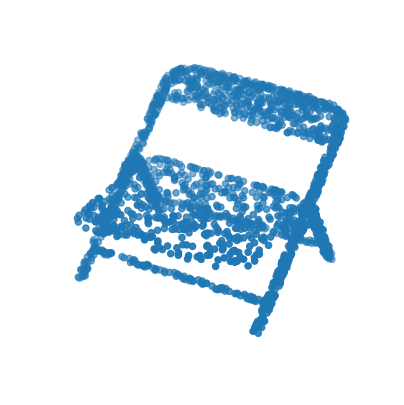
To convert a mesh file to a point cloud we first need to sample points on the mesh surface. .sample() performs a uniform random sampling. Here we sample at 2048 locations and visualize in matplotlib.
points = mesh.sample(2048)

fig = plt.figure(figsize=(5, 5))
ax = fig.add_subplot(111, projection="3d")
ax.scatter(points[:, 0], points[:, 1], points[:, 2])
ax.set_axis_off()
plt.show()
To generate a tf.data.Dataset() we need to first parse through the ModelNet data folders. Each mesh is loaded and sampled into a point cloud before being added to a standard python list and converted to a numpy array. We also store the current enumerate index value as the object label and use a dictionary to recall this later.
def parse_dataset(num_points=2048):
    train_points = []
    train_labels = []
    test_points = []
    test_labels = []
    class_map = {}
    folders = glob.glob(os.path.join(DATA_DIR, "[!README]*"))

    for i, folder in enumerate(folders):
        print("processing class: {}".format(os.path.basename(folder)))
        # store folder name with ID so we can retrieve later
        class_map[i] = folder.split("/")[-1]
        # gather all files
        train_files = glob.glob(os.path.join(folder, "train/*"))
        test_files = glob.glob(os.path.join(folder, "test/*"))

        for f in train_files:
            train_points.append(trimesh.load(f).sample(num_points))
            train_labels.append(i)

        for f in test_files:
            test_points.append(trimesh.load(f).sample(num_points))
            test_labels.append(i)

    return (
        np.array(train_points),
        np.array(test_points),
        np.array(train_labels),
        np.array(test_labels),
        class_map,
    )
Set the number of points to sample and batch size and parse the dataset. This can take ~5minutes to complete.
NUM_POINTS = 2048
NUM_CLASSES = 10
BATCH_SIZE = 32

train_points, test_points, train_labels, test_labels, CLASS_MAP = parse_dataset(
    NUM_POINTS
)
processing class: bathtub

processing class: monitor

processing class: desk

processing class: dresser

processing class: toilet

processing class: bed

processing class: sofa

processing class: chair

processing class: night_stand

processing class: table
Our data can now be read into a tf.data.Dataset() object. We set the shuffle buffer size to the entire size of the dataset as prior to this the data is ordered by class. Data augmentation is important when working with point cloud data. We create a augmentation function to jitter and shuffle the train dataset.
def augment(points, label):
    # jitter points
    points += keras.random.uniform(points.shape, -0.005, 0.005, dtype="float64")
    # shuffle points
    points = keras.random.shuffle(points)
    return points, label


train_size = 0.8
dataset = tf_data.Dataset.from_tensor_slices((train_points, train_labels))
test_dataset = tf_data.Dataset.from_tensor_slices((test_points, test_labels))
train_dataset_size = int(len(dataset) * train_size)

dataset = dataset.shuffle(len(train_points)).map(augment)
test_dataset = test_dataset.shuffle(len(test_points)).batch(BATCH_SIZE)

train_dataset = dataset.take(train_dataset_size).batch(BATCH_SIZE)
validation_dataset = dataset.skip(train_dataset_size).batch(BATCH_SIZE)
Build a model
Each convolution and fully-connected layer (with exception for end layers) consists of Convolution / Dense -> Batch Normalization -> ReLU Activation.
def conv_bn(x, filters):
    x = layers.Conv1D(filters, kernel_size=1, padding="valid")(x)
    x = layers.BatchNormalization(momentum=0.0)(x)
    return layers.Activation("relu")(x)


def dense_bn(x, filters):
    x = layers.Dense(filters)(x)
    x = layers.BatchNormalization(momentum=0.0)(x)
    return layers.Activation("relu")(x)
| PointNet consists of two core components. The primary MLP network, and the transformer net (T-net). The T-net aims to learn an affine transformation matrix by its own mini network. The T-net is used twice. The first time to transform the input features (n, 3) into a canonical representation. The second is an affine transformation for alignment in feature space (n, 3). As per the original paper we constrain the transformation to be close to an orthogonal matrix (i.e. | X*X^T - I | = 0). |
class OrthogonalRegularizer(keras.regularizers.Regularizer):
    def __init__(self, num_features, l2reg=0.001):
        self.num_features = num_features
        self.l2reg = l2reg
        self.eye = ops.eye(num_features)

    def __call__(self, x):
        x = ops.reshape(x, (-1, self.num_features, self.num_features))
        xxt = ops.tensordot(x, x, axes=(2, 2))
        xxt = ops.reshape(xxt, (-1, self.num_features, self.num_features))
        return ops.sum(self.l2reg * ops.square(xxt - self.eye))
We can then define a general function to build T-net layers.
def tnet(inputs, num_features):
    # Initialise bias as the identity matrix
    bias = keras.initializers.Constant(np.eye(num_features).flatten())
    reg = OrthogonalRegularizer(num_features)

    x = conv_bn(inputs, 32)
    x = conv_bn(x, 64)
    x = conv_bn(x, 512)
    x = layers.GlobalMaxPooling1D()(x)
    x = dense_bn(x, 256)
    x = dense_bn(x, 128)
    x = layers.Dense(
        num_features * num_features,
        kernel_initializer="zeros",
        bias_initializer=bias,
        activity_regularizer=reg,
    )(x)
    feat_T = layers.Reshape((num_features, num_features))(x)
    # Apply affine transformation to input features
    return layers.Dot(axes=(2, 1))([inputs, feat_T])
The main network can be then implemented in the same manner where the t-net mini models can be dropped in a layers in the graph. Here we replicate the network architecture published in the original paper but with half the number of weights at each layer as we are using the smaller 10 class ModelNet dataset.
inputs = keras.Input(shape=(NUM_POINTS, 3))

x = tnet(inputs, 3)
x = conv_bn(x, 32)
x = conv_bn(x, 32)
x = tnet(x, 32)
x = conv_bn(x, 32)
x = conv_bn(x, 64)
x = conv_bn(x, 512)
x = layers.GlobalMaxPooling1D()(x)
x = dense_bn(x, 256)
x = layers.Dropout(0.3)(x)
x = dense_bn(x, 128)
x = layers.Dropout(0.3)(x)

outputs = layers.Dense(NUM_CLASSES, activation="softmax")(x)

model = keras.Model(inputs=inputs, outputs=outputs, name="pointnet")
model.summary()
Model: "pointnet"
┏━━━━━━━━━━━━━━━━━━━━━┳━━━━━━━━━━━━━━━━━━━┳━━━━━━━━━┳━━━━━━━━━━━━━━━━━━━━━━┓
┃ Layer (type)        ┃ Output Shape      ┃ Param # ┃ Connected to         ┃
┡━━━━━━━━━━━━━━━━━━━━━╇━━━━━━━━━━━━━━━━━━━╇━━━━━━━━━╇━━━━━━━━━━━━━━━━━━━━━━┩
│ input_layer         │ (None, 2048, 3)   │       0 │ -                    │
│ (InputLayer)        │                   │         │                      │
├─────────────────────┼───────────────────┼─────────┼──────────────────────┤
│ conv1d (Conv1D)     │ (None, 2048, 32)  │     128 │ input_layer[0][0]    │
├─────────────────────┼───────────────────┼─────────┼──────────────────────┤
│ batch_normalization │ (None, 2048, 32)  │     128 │ conv1d[0][0]         │
│ (BatchNormalizatio… │                   │         │                      │
├─────────────────────┼───────────────────┼─────────┼──────────────────────┤
│ activation          │ (None, 2048, 32)  │       0 │ batch_normalization… │
│ (Activation)        │                   │         │                      │
├─────────────────────┼───────────────────┼─────────┼──────────────────────┤
│ conv1d_1 (Conv1D)   │ (None, 2048, 64)  │   2,112 │ activation[0][0]     │
├─────────────────────┼───────────────────┼─────────┼──────────────────────┤
│ batch_normalizatio… │ (None, 2048, 64)  │     256 │ conv1d_1[0][0]       │
│ (BatchNormalizatio… │                   │         │                      │
├─────────────────────┼───────────────────┼─────────┼──────────────────────┤
│ activation_1        │ (None, 2048, 64)  │       0 │ batch_normalization… │
│ (Activation)        │                   │         │                      │
├─────────────────────┼───────────────────┼─────────┼──────────────────────┤
│ conv1d_2 (Conv1D)   │ (None, 2048, 512) │  33,280 │ activation_1[0][0]   │
├─────────────────────┼───────────────────┼─────────┼──────────────────────┤
│ batch_normalizatio… │ (None, 2048, 512) │   2,048 │ conv1d_2[0][0]       │
│ (BatchNormalizatio… │                   │         │                      │
├─────────────────────┼───────────────────┼─────────┼──────────────────────┤
│ activation_2        │ (None, 2048, 512) │       0 │ batch_normalization… │
│ (Activation)        │                   │         │                      │
├─────────────────────┼───────────────────┼─────────┼──────────────────────┤
│ global_max_pooling… │ (None, 512)       │       0 │ activation_2[0][0]   │
│ (GlobalMaxPooling1… │                   │         │                      │
├─────────────────────┼───────────────────┼─────────┼──────────────────────┤
│ dense (Dense)       │ (None, 256)       │ 131,328 │ global_max_pooling1… │
├─────────────────────┼───────────────────┼─────────┼──────────────────────┤
│ batch_normalizatio… │ (None, 256)       │   1,024 │ dense[0][0]          │
│ (BatchNormalizatio… │                   │         │                      │
├─────────────────────┼───────────────────┼─────────┼──────────────────────┤
│ activation_3        │ (None, 256)       │       0 │ batch_normalization… │
│ (Activation)        │                   │         │                      │
├─────────────────────┼───────────────────┼─────────┼──────────────────────┤
│ dense_1 (Dense)     │ (None, 128)       │  32,896 │ activation_3[0][0]   │
├─────────────────────┼───────────────────┼─────────┼──────────────────────┤
│ batch_normalizatio… │ (None, 128)       │     512 │ dense_1[0][0]        │
│ (BatchNormalizatio… │                   │         │                      │
├─────────────────────┼───────────────────┼─────────┼──────────────────────┤
│ activation_4        │ (None, 128)       │       0 │ batch_normalization… │
│ (Activation)        │                   │         │                      │
├─────────────────────┼───────────────────┼─────────┼──────────────────────┤
│ dense_2 (Dense)     │ (None, 9)         │   1,161 │ activation_4[0][0]   │
├─────────────────────┼───────────────────┼─────────┼──────────────────────┤
│ reshape (Reshape)   │ (None, 3, 3)      │       0 │ dense_2[0][0]        │
├─────────────────────┼───────────────────┼─────────┼──────────────────────┤
│ dot (Dot)           │ (None, 2048, 3)   │       0 │ input_layer[0][0],   │
│                     │                   │         │ reshape[0][0]        │
├─────────────────────┼───────────────────┼─────────┼──────────────────────┤
│ conv1d_3 (Conv1D)   │ (None, 2048, 32)  │     128 │ dot[0][0]            │
├─────────────────────┼───────────────────┼─────────┼──────────────────────┤
│ batch_normalizatio… │ (None, 2048, 32)  │     128 │ conv1d_3[0][0]       │
│ (BatchNormalizatio… │                   │         │                      │
├─────────────────────┼───────────────────┼─────────┼──────────────────────┤
│ activation_5        │ (None, 2048, 32)  │       0 │ batch_normalization… │
│ (Activation)        │                   │         │                      │
├─────────────────────┼───────────────────┼─────────┼──────────────────────┤
│ conv1d_4 (Conv1D)   │ (None, 2048, 32)  │   1,056 │ activation_5[0][0]   │
├─────────────────────┼───────────────────┼─────────┼──────────────────────┤
│ batch_normalizatio… │ (None, 2048, 32)  │     128 │ conv1d_4[0][0]       │
│ (BatchNormalizatio… │                   │         │                      │
├─────────────────────┼───────────────────┼─────────┼──────────────────────┤
│ activation_6        │ (None, 2048, 32)  │       0 │ batch_normalization… │
│ (Activation)        │                   │         │                      │
├─────────────────────┼───────────────────┼─────────┼──────────────────────┤
│ conv1d_5 (Conv1D)   │ (None, 2048, 32)  │   1,056 │ activation_6[0][0]   │
├─────────────────────┼───────────────────┼─────────┼──────────────────────┤
│ batch_normalizatio… │ (None, 2048, 32)  │     128 │ conv1d_5[0][0]       │
│ (BatchNormalizatio… │                   │         │                      │
├─────────────────────┼───────────────────┼─────────┼──────────────────────┤
│ activation_7        │ (None, 2048, 32)  │       0 │ batch_normalization… │
│ (Activation)        │                   │         │                      │
├─────────────────────┼───────────────────┼─────────┼──────────────────────┤
│ conv1d_6 (Conv1D)   │ (None, 2048, 64)  │   2,112 │ activation_7[0][0]   │
├─────────────────────┼───────────────────┼─────────┼──────────────────────┤
│ batch_normalizatio… │ (None, 2048, 64)  │     256 │ conv1d_6[0][0]       │
│ (BatchNormalizatio… │                   │         │                      │
├─────────────────────┼───────────────────┼─────────┼──────────────────────┤
│ activation_8        │ (None, 2048, 64)  │       0 │ batch_normalization… │
│ (Activation)        │                   │         │                      │
├─────────────────────┼───────────────────┼─────────┼──────────────────────┤
│ conv1d_7 (Conv1D)   │ (None, 2048, 512) │  33,280 │ activation_8[0][0]   │
├─────────────────────┼───────────────────┼─────────┼──────────────────────┤
│ batch_normalizatio… │ (None, 2048, 512) │   2,048 │ conv1d_7[0][0]       │
│ (BatchNormalizatio… │                   │         │                      │
├─────────────────────┼───────────────────┼─────────┼──────────────────────┤
│ activation_9        │ (None, 2048, 512) │       0 │ batch_normalization… │
│ (Activation)        │                   │         │                      │
├─────────────────────┼───────────────────┼─────────┼──────────────────────┤
│ global_max_pooling… │ (None, 512)       │       0 │ activation_9[0][0]   │
│ (GlobalMaxPooling1… │                   │         │                      │
├─────────────────────┼───────────────────┼─────────┼──────────────────────┤
│ dense_3 (Dense)     │ (None, 256)       │ 131,328 │ global_max_pooling1… │
├─────────────────────┼───────────────────┼─────────┼──────────────────────┤
│ batch_normalizatio… │ (None, 256)       │   1,024 │ dense_3[0][0]        │
│ (BatchNormalizatio… │                   │         │                      │
├─────────────────────┼───────────────────┼─────────┼──────────────────────┤
│ activation_10       │ (None, 256)       │       0 │ batch_normalization… │
│ (Activation)        │                   │         │                      │
├─────────────────────┼───────────────────┼─────────┼──────────────────────┤
│ dense_4 (Dense)     │ (None, 128)       │  32,896 │ activation_10[0][0]  │
├─────────────────────┼───────────────────┼─────────┼──────────────────────┤
│ batch_normalizatio… │ (None, 128)       │     512 │ dense_4[0][0]        │
│ (BatchNormalizatio… │                   │         │                      │
├─────────────────────┼───────────────────┼─────────┼──────────────────────┤
│ activation_11       │ (None, 128)       │       0 │ batch_normalization… │
│ (Activation)        │                   │         │                      │
├─────────────────────┼───────────────────┼─────────┼──────────────────────┤
│ dense_5 (Dense)     │ (None, 1024)      │ 132,096 │ activation_11[0][0]  │
├─────────────────────┼───────────────────┼─────────┼──────────────────────┤
│ reshape_1 (Reshape) │ (None, 32, 32)    │       0 │ dense_5[0][0]        │
├─────────────────────┼───────────────────┼─────────┼──────────────────────┤
│ dot_1 (Dot)         │ (None, 2048, 32)  │       0 │ activation_6[0][0],  │
│                     │                   │         │ reshape_1[0][0]      │
├─────────────────────┼───────────────────┼─────────┼──────────────────────┤
│ conv1d_8 (Conv1D)   │ (None, 2048, 32)  │   1,056 │ dot_1[0][0]          │
├─────────────────────┼───────────────────┼─────────┼──────────────────────┤
│ batch_normalizatio… │ (None, 2048, 32)  │     128 │ conv1d_8[0][0]       │
│ (BatchNormalizatio… │                   │         │                      │
├─────────────────────┼───────────────────┼─────────┼──────────────────────┤
│ activation_12       │ (None, 2048, 32)  │       0 │ batch_normalization… │
│ (Activation)        │                   │         │                      │
├─────────────────────┼───────────────────┼─────────┼──────────────────────┤
│ conv1d_9 (Conv1D)   │ (None, 2048, 64)  │   2,112 │ activation_12[0][0]  │
├─────────────────────┼───────────────────┼─────────┼──────────────────────┤
│ batch_normalizatio… │ (None, 2048, 64)  │     256 │ conv1d_9[0][0]       │
│ (BatchNormalizatio… │                   │         │                      │
├─────────────────────┼───────────────────┼─────────┼──────────────────────┤
│ activation_13       │ (None, 2048, 64)  │       0 │ batch_normalization… │
│ (Activation)        │                   │         │                      │
├─────────────────────┼───────────────────┼─────────┼──────────────────────┤
│ conv1d_10 (Conv1D)  │ (None, 2048, 512) │  33,280 │ activation_13[0][0]  │
├─────────────────────┼───────────────────┼─────────┼──────────────────────┤
│ batch_normalizatio… │ (None, 2048, 512) │   2,048 │ conv1d_10[0][0]      │
│ (BatchNormalizatio… │                   │         │                      │
├─────────────────────┼───────────────────┼─────────┼──────────────────────┤
│ activation_14       │ (None, 2048, 512) │       0 │ batch_normalization… │
│ (Activation)        │                   │         │                      │
├─────────────────────┼───────────────────┼─────────┼──────────────────────┤
│ global_max_pooling… │ (None, 512)       │       0 │ activation_14[0][0]  │
│ (GlobalMaxPooling1… │                   │         │                      │
├─────────────────────┼───────────────────┼─────────┼──────────────────────┤
│ dense_6 (Dense)     │ (None, 256)       │ 131,328 │ global_max_pooling1… │
├─────────────────────┼───────────────────┼─────────┼──────────────────────┤
│ batch_normalizatio… │ (None, 256)       │   1,024 │ dense_6[0][0]        │
│ (BatchNormalizatio… │                   │         │                      │
├─────────────────────┼───────────────────┼─────────┼──────────────────────┤
│ activation_15       │ (None, 256)       │       0 │ batch_normalization… │
│ (Activation)        │                   │         │                      │
├─────────────────────┼───────────────────┼─────────┼──────────────────────┤
│ dropout (Dropout)   │ (None, 256)       │       0 │ activation_15[0][0]  │
├─────────────────────┼───────────────────┼─────────┼──────────────────────┤
│ dense_7 (Dense)     │ (None, 128)       │  32,896 │ dropout[0][0]        │
├─────────────────────┼───────────────────┼─────────┼──────────────────────┤
│ batch_normalizatio… │ (None, 128)       │     512 │ dense_7[0][0]        │
│ (BatchNormalizatio… │                   │         │                      │
├─────────────────────┼───────────────────┼─────────┼──────────────────────┤
│ activation_16       │ (None, 128)       │       0 │ batch_normalization… │
│ (Activation)        │                   │         │                      │
├─────────────────────┼───────────────────┼─────────┼──────────────────────┤
│ dropout_1 (Dropout) │ (None, 128)       │       0 │ activation_16[0][0]  │
├─────────────────────┼───────────────────┼─────────┼──────────────────────┤
│ dense_8 (Dense)     │ (None, 10)        │   1,290 │ dropout_1[0][0]      │
└─────────────────────┴───────────────────┴─────────┴──────────────────────┘
 Total params: 748,979 (2.86 MB)
 Trainable params: 742,899 (2.83 MB)
 Non-trainable params: 6,080 (23.75 KB)
Train model
Once the model is defined it can be trained like any other standard classification model using .compile() and .fit().
model.compile(
    loss="sparse_categorical_crossentropy",
    optimizer=keras.optimizers.Adam(learning_rate=0.001),
    metrics=["sparse_categorical_accuracy"],
)

model.fit(train_dataset, epochs=20, validation_data=validation_dataset)
Epoch 1/20
1/100 [37m━━━━━━━━━━━━━━━━━━━━ 16:59 10s/step - loss: 70.7465 - sparse_categorical_accuracy: 0.2188
100/100 ━━━━━━━━━━━━━━━━━━━━ 119s 1s/step - loss: 45.9764 - sparse_categorical_accuracy: 0.2156 - val_loss: 4122951.0000 - val_sparse_categorical_accuracy: 0.3154
Epoch 2/20
1/100 [37m━━━━━━━━━━━━━━━━━━━━ 1:44 1s/step - loss: 36.7920 - sparse_categorical_accuracy: 0.2500
100/100 ━━━━━━━━━━━━━━━━━━━━ 108s 1s/step - loss: 36.6386 - sparse_categorical_accuracy: 0.2751 - val_loss: 20961250112658389073920.0000 - val_sparse_categorical_accuracy: 0.3191
Epoch 3/20
1/100 [37m━━━━━━━━━━━━━━━━━━━━ 57:33 35s/step - loss: 35.9745 - sparse_categorical_accuracy: 0.3438
100/100 ━━━━━━━━━━━━━━━━━━━━ 142s 1s/step - loss: 36.4148 - sparse_categorical_accuracy: 0.3150 - val_loss: 14661139300352.0000 - val_sparse_categorical_accuracy: 0.2240
Epoch 4/20
1/100 [37m━━━━━━━━━━━━━━━━━━━━ 1:40 1s/step - loss: 36.7380 - sparse_categorical_accuracy: 0.5312
100/100 ━━━━━━━━━━━━━━━━━━━━ 110s 1s/step - loss: 36.7658 - sparse_categorical_accuracy: 0.3286 - val_loss: 2640681721921536.0000 - val_sparse_categorical_accuracy: 0.3542
Epoch 5/20
1/100 [37m━━━━━━━━━━━━━━━━━━━━ 1:43 1s/step - loss: 36.6004 - sparse_categorical_accuracy: 0.2188
100/100 ━━━━━━━━━━━━━━━━━━━━ 112s 1s/step - loss: 36.9928 - sparse_categorical_accuracy: 0.3100 - val_loss: 2087371157504536015273984.0000 - val_sparse_categorical_accuracy: 0.3004
Epoch 6/20
1/100 [37m━━━━━━━━━━━━━━━━━━━━ 1:43 1s/step - loss: 37.1168 - sparse_categorical_accuracy: 0.1875
100/100 ━━━━━━━━━━━━━━━━━━━━ 108s 1s/step - loss: 36.6758 - sparse_categorical_accuracy: 0.3182 - val_loss: 598952362161209344.0000 - val_sparse_categorical_accuracy: 0.4180
Epoch 7/20
1/100 [37m━━━━━━━━━━━━━━━━━━━━ 1:46 1s/step - loss: 36.5799 - sparse_categorical_accuracy: 0.2188
100/100 ━━━━━━━━━━━━━━━━━━━━ 107s 1s/step - loss: 37.8231 - sparse_categorical_accuracy: 0.3192 - val_loss: 1330149064704.0000 - val_sparse_categorical_accuracy: 0.3367
Epoch 8/20
1/100 [37m━━━━━━━━━━━━━━━━━━━━ 1:42 1s/step - loss: 36.6512 - sparse_categorical_accuracy: 0.2500
100/100 ━━━━━━━━━━━━━━━━━━━━ 107s 1s/step - loss: 36.4611 - sparse_categorical_accuracy: 0.3198 - val_loss: 55461990629376.0000 - val_sparse_categorical_accuracy: 0.3805
Epoch 9/20
1/100 [37m━━━━━━━━━━━━━━━━━━━━ 1:48 1s/step - loss: 36.1902 - sparse_categorical_accuracy: 0.4062\
100/100 ━━━━━━━━━━━━━━━━━━━━ 107s 1s/step - loss: 36.3207 - sparse_categorical_accuracy: 0.3371 - val_loss: 79361986265088.0000 - val_sparse_categorical_accuracy: 0.3680
Epoch 10/20
1/100 [37m━━━━━━━━━━━━━━━━━━━━ 58:50 36s/step - loss: 36.7173 - sparse_categorical_accuracy: 0.4062
100/100 ━━━━━━━━━━━━━━━━━━━━ 142s 1s/step - loss: 36.0947 - sparse_categorical_accuracy: 0.3475 - val_loss: 14927241216.0000 - val_sparse_categorical_accuracy: 0.3054
Epoch 11/20
1/100 [37m━━━━━━━━━━━━━━━━━━━━ 58:42 36s/step - loss: 36.1768 - sparse_categorical_accuracy: 0.3438
100/100 ━━━━━━━━━━━━━━━━━━━━ 141s 1s/step - loss: 38.5024 - sparse_categorical_accuracy: 0.3187 - val_loss: 1930753792.0000 - val_sparse_categorical_accuracy: 0.2315
Epoch 12/20
1/100 [37m━━━━━━━━━━━━━━━━━━━━ 1:00:07 36s/step - loss: 42.1152 - sparse_categorical_accuracy: 0.3750
100/100 ━━━━━━━━━━━━━━━━━━━━ 142s 1s/step - loss: 37.4206 - sparse_categorical_accuracy: 0.3256 - val_loss: 1793616557963500563988480.0000 - val_sparse_categorical_accuracy: 0.2328
Epoch 13/20
1/100 [37m━━━━━━━━━━━━━━━━━━━━ 59:52 36s/step - loss: 43.0665 - sparse_categorical_accuracy: 0.1875
100/100 ━━━━━━━━━━━━━━━━━━━━ 142s 1s/step - loss: 56.5366 - sparse_categorical_accuracy: 0.3226 - val_loss: 505209651200.0000 - val_sparse_categorical_accuracy: 0.2528
Epoch 14/20
1/100 [37m━━━━━━━━━━━━━━━━━━━━ 1:46 1s/step - loss: 72.5004 - sparse_categorical_accuracy: 0.2812
100/100 ━━━━━━━━━━━━━━━━━━━━ 107s 1s/step - loss: 407.6649 - sparse_categorical_accuracy: 0.3007 - val_loss: 35970580884750336.0000 - val_sparse_categorical_accuracy: 0.3392
Epoch 15/20
1/100 [37m━━━━━━━━━━━━━━━━━━━━ 1:41 1s/step - loss: 67.1360 - sparse_categorical_accuracy: 0.1875
100/100 ━━━━━━━━━━━━━━━━━━━━ 106s 1s/step - loss: 77.4712 - sparse_categorical_accuracy: 0.3377 - val_loss: 2983669504.0000 - val_sparse_categorical_accuracy: 0.2966
Epoch 16/20
1/100 [37m━━━━━━━━━━━━━━━━━━━━ 1:38 992ms/step - loss: 59.8730 - sparse_categorical_accuracy: 0.2188
100/100 ━━━━━━━━━━━━━━━━━━━━ 107s 1s/step - loss: 67.4222 - sparse_categorical_accuracy: 0.3189 - val_loss: 37.0687 - val_sparse_categorical_accuracy: 0.1477
Epoch 17/20
1/100 [37m━━━━━━━━━━━━━━━━━━━━ 58:50 36s/step - loss: 54.1712 - sparse_categorical_accuracy: 0.5312
100/100 ━━━━━━━━━━━━━━━━━━━━ 141s 1s/step - loss: 58.2869 - sparse_categorical_accuracy: 0.3282 - val_loss: 4191578574815232.0000 - val_sparse_categorical_accuracy: 0.3129
Epoch 18/20
1/100 [37m━━━━━━━━━━━━━━━━━━━━ 1:39 1s/step - loss: 51.9365 - sparse_categorical_accuracy: 0.4375
100/100 ━━━━━━━━━━━━━━━━━━━━ 106s 1s/step - loss: 55.1443 - sparse_categorical_accuracy: 0.3351 - val_loss: 50221851662203486208.0000 - val_sparse_categorical_accuracy: 0.3242
Epoch 19/20
1/100 [37m━━━━━━━━━━━━━━━━━━━━ 1:41 1s/step - loss: 48.0290 - sparse_categorical_accuracy: 0.2188
100/100 ━━━━━━━━━━━━━━━━━━━━ 108s 1s/step - loss: 49.9001 - sparse_categorical_accuracy: 0.3317 - val_loss: 69256328.0000 - val_sparse_categorical_accuracy: 0.3579
Epoch 20/20
1/100 [37m━━━━━━━━━━━━━━━━━━━━ 1:42 1s/step - loss: 45.8100 - sparse_categorical_accuracy: 0.4062
100/100 ━━━━━━━━━━━━━━━━━━━━ 106s 1s/step - loss: 47.4913 - sparse_categorical_accuracy: 0.3404 - val_loss: 1814011445248.0000 - val_sparse_categorical_accuracy: 0.3592
<keras.src.callbacks.history.History at 0x7f596cb7b8e0>
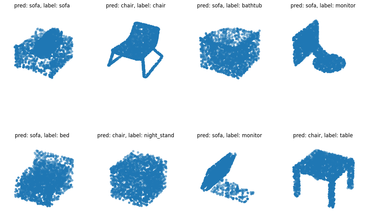
Visualize predictions
We can use matplotlib to visualize our trained model performance.
data = test_dataset.take(1)

points, labels = list(data)[0]
points = points[:8, ...]
labels = labels[:8, ...]

# run test data through model
preds = model.predict(points)
preds = ops.argmax(preds, -1)

points = points.numpy()

# plot points with predicted class and label
fig = plt.figure(figsize=(15, 10))
for i in range(8):
    ax = fig.add_subplot(2, 4, i + 1, projection="3d")
    ax.scatter(points[i, :, 0], points[i, :, 1], points[i, :, 2])
    ax.set_title(
        "pred: {:}, label: {:}".format(
            CLASS_MAP[preds[i].numpy()], CLASS_MAP[labels.numpy()[i]]
        )
    )
    ax.set_axis_off()
plt.show()
1/1 ━━━━━━━━━━━━━━━━━━━━ 0s 404ms/step
1/1 ━━━━━━━━━━━━━━━━━━━━ 0s 405ms/step